[Update 2022 Dec. 4] Added contrastive learning / decoding methods.
[Update 2023 Mar. 10] Refactor and adding RLHF and diffusion methods.
[Update 2023 Dec. 22] Added DPO, RAG and EMNLP 2023 papers.
Intro
The task of generating content from deep learning models is different from other common tasks in the sens that 1) the model is often trained to replicate the training data for continuous models or predict the next element for discrete ones; 2) when testing a model, there is no exact expected results, in consequence; 3) its evaluation is often tricky.
The underlying objective is to train a model so it can generate realistic content during inference. For continuous domains, state of the art models are mostly based on adversarial (Generative Adversarial Networks, GANs) and denoising diffusion training objectives. These models are capable to create impressive and highly realistic results in a wide variety of styles. For discrete domains, generative tasks are commonly performed by sequential models, that are trained with teacher forcing and used autoregressively during inference (generate elements one after another). This discrepancy between training objective and inference procedure often make results to degenerate: the model falls in a loops where it repetitively predicts the same sentence, and/or drifts from the initial topic. This problem is known as exposure bias.
Alleviating the effects of the exposure bias is a whole research area, in which researchers introduced generation methods intending to select the best next-token. Other researchers believe that autoregressive generation is by nature doomed to be subject to exposure bias no matter what decoding technique is employed. Gradient based methods such as diffusion models (and some extent Generative Adversarial Networks) are indeed very appealing for any generative purpose. They are however by nature not suited to be employed for discrete modalities without significant design changes. Attempts to adapt these methods for natural language have been shown to work, but are in practice not practical to train and not on par (yet?) with their autoregressive counterparts.
We will take a look to all these solutions, which goes beyond teacher forcing and autoregressive inference.
Problem formulation
Let’s formulate the problem before going further.
| Symbol | Meaning |
|---|---|
| $g_\theta$ | Generator network with parameters $\theta$ |
| $d_\delta$ | Discriminator network with parameters $\delta$ |
| $p_d$ | Data distribution over real samples |
| $\mathbf{x} \in \mathbb{R}^L$ | A real sample $\sim p_d(\mathbf{x})$ |
| $p_\theta$ | Model distribution over generated samples |
| $p_z$ | Data distribution over Gaussian noise / latent space |
| $\mathbf{z} \in \mathbb{R}^L$ | Latent variable sampled from the latent space $\sim p_z(\mathbf{z})$ |
| $\mathcal{V}$ | The vocabulary set, linking each token (or integer index) to its word / subword / meaning |
| $V$ | Size of the vocabulary, with $\lvert \mathcal{V} \lvert = V$ |
The objective of a training model is to generate content that is realistic, thus similar (not identical) to the data it was trained on. This objective can be expressed as $\underset{\theta}{\mathrm{min}}\: \mathrm{KL}(p_\theta \lvert\lvert p_d)$ where we want the model distribution to be the closest possible to the data distribution.
A generative model is ideally trained to reflect this objective.
The exposure bias
Sequential models are trained on Maximum Likelihood Estimation (MLE), and have a training objective expressed as $\mathrm{max}\: \mathbb{E}_{\mathbf{x} \sim p_d(\mathbf{x})} [log \left( g_\theta (\mathbf{x}) \right)]$. Yet, during inference they are used autoregressively to generate content, as $g_{\theta} \left( \mathbf{x} \right) = \prod_{t=1}^{T} g_{\theta} \left( x_t \lvert \mathbf{x}_{<t} \right)$. As the inference step $t$ progresses, the model is increasingly likely to predict incoherent or repetitive tokens which can deviate from the original context. This text degeneration issue is commonly called exposure bias.
Autoregressive decoding methods
Top-k / nucleus / greedy sampling
Greedy decoding, which consist in picking the token with the highest probability score given by the model, is known to be very prone to repetitions and text degeneration. Stochastic decodings help to reduce these effects. The two most used methods are top-k sampling and nucleus sampling. Here is a very good post which goes into details on these techniques. We will see here more complex decoding methods.
NeuroLogic
Some NLG tasks require to impose some constraints on the generated sequence. For instance the generation of a recipe from a list of ingredients. On top one could also desire to not predict specific output words / tokens. The commonly used technique is to fine-tune a large pre-trained model on task-specific datasets. Doing so, the model however do not learn to effectively satisfy the constraints and often struggles with new constraints and few or zero-shot tasks. The underlying task is then to find an optimal output sequence which satisfies the constraints while having high likelihoods for each element within. NeuroLogic addresses this issue by converting the constraints into penalties during the decoding process. It uses beam-search to generate multiple sequences and steer them toward predictions with low penalties.
The authors enumerate four states that each constraint can take during the decoding: reversible unsatisfaction, irreversible unsatisfaction, reversible satisfaction and irreversible satisfaction. At each decoding step, the model distribution of each beam ($\in \mathbb{R}^{V}$) are modified to: 1) discard tokens leading to irreversible unsatisfaction; 2) keep only tokens with the top-k likelihoods and top-$\beta$ in term of satisfied constraints; 3) group the remaining tokens by constraint satisfied. Within each group, each token is assigned a score $s = p_\theta(y_t \lvert \mathbf{y}_{<t}) + \lambda \underset{D(c_i, \mathbf{y}_{0:t})}{max} \frac{\hat{c_i}}{c_i}$ where $\lambda$ is an adjustable parameter, $c_i$ is the number of successive tokens the constraint $i$ contains, $\hat{c_i}$ is the number of tokens already predicted of the $i$, $D(c_i, \mathbf{y})$ means the constraint $c_i$ is satisfied by $\mathbf{y}$. The token with the highest score is selected for each beam. The NeuroLogic technique achieved SOTA ROUGE and BLEU results on conditional text generation tasks such as CommonGen.
NeuroLogic A*esque relies on NeuroLogic and adds an A* search heuristic on top to estimate the score of the tokens at each decoding step. The score of the token $v$ at decoding step $t$ is calculated as $f(y_{t,v}) = s(\mathbf{y}_{<t}) + h(y_{t,v})$ where $s(\mathbf{y}_{<t})$ is the decoded sequence so far and $h(y_{t,v})$ is a estimation of the score of the future sequence. In practice, $h(y_{t,v})$ is computed by generating a beam search continuation of $l$ tokens in the future. Each continuation is then evaluated by the Neurologic score formula, which consider user defined constraints.
GANs for natural language generation
Generative Adversarial Networks are a class of models featuring a generator and a discriminator, both trained adversarially. We will see here how they work, why they work well for continuous modalities such as images, but not much for discrete ones like natural language. Despite this, several attempts have been made and successfully generate coherent text results in certain conditions.
A GAN is made of two networks:
- A generator $g_\theta$ which takes random Gaussian noise $\mathbf{z}$ as input, and produces an output $\mathbf{y}$;
- A discriminator $d_\delta$ which tells if its input is wether fake or real.
The role of the generator is to create content close to a real data distribution $p_d$, while the discriminator must tell apart real samples from fake ones created by the generator.
Schema of a GAN training procedure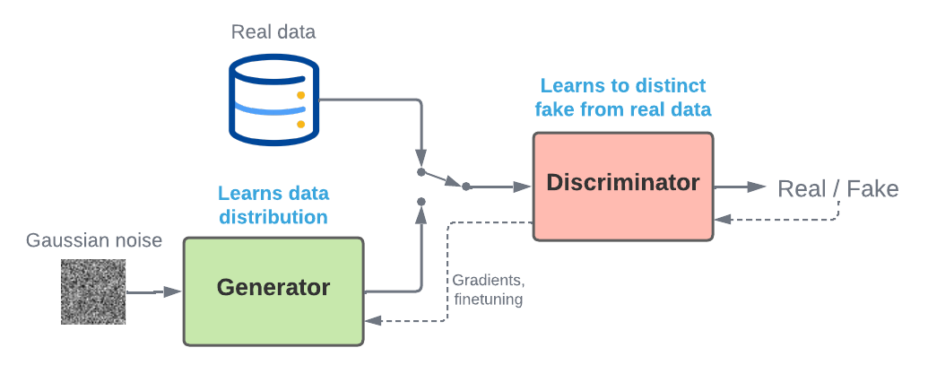
During training, when the discriminator fails, its parameters $\delta$ are updated. It is trained to maximize it’s result over real data $\mathrm{max}: \mathbb{E}_{\mathbf{x} \sim p_x(\mathbf{x})} [log \left( d_\delta (\mathbf{x}) \right)]$, while minimizing the prediction of generated samples $g_\theta (\mathbf{z})$, $\mathrm{min}: \mathbb{E}_{\mathbf{z} \sim p_z(\mathbf{z})} [log \left( 1 - d_\delta (g_\theta (\mathbf{z})) \right)]$.
When the discriminator succeeds, the generator’s parameters $\theta$ are updated. It is trained to generate samples which maximize their result from the discriminator (fools it), hence minimizing $\mathbb{E}_{\mathbf{z} \sim p_z(\mathbf{z})} [log \left( 1 - d_\delta (g_\theta (\mathbf{z})) \right)]$.
This can in turn be written as: $$\underset{\theta}{\mathrm{min}}\: \underset{\delta}{\mathrm{max}}\: \mathcal{L}(g_\theta, d_\delta) = \mathbb{E}_{x \sim p_x(\mathbf{x})} [\mathrm{log}: d_\delta(x)] + \mathbb{E}_{z \sim p_z(\mathbf{z})} [\mathrm{log} (1 - d_\delta(g_\theta(\mathbf{z})))]$$
The generator will progressively produce content closer to $p_d$, and the discriminator will distinguish real from fake data with smaller differences. Both models are jointly trained, improving each other.
You see that the generator is directly trained to minimize the distance between its distribution and the data distribution: $\underset{\theta}{\mathrm{min}}\: \mathrm{KL}(p_\theta \lvert\lvert p_d)$. This allows to generate original content which contains the underlying features of the data distribution implicitly.
Why not for discrete data ?
GANs have essentially been applied to continuous domains so far. The reason is because the output of the generator $\mathbf{y}$ is the input of the discriminator, thus every operation in between must be differentiable. Sequential models however return discrete distributions, from which we would have to sample $\mathbf{y} \sim g_\theta \left( \mathbf{x} \right)$ in order to estimate the result and pass it to the discriminator. But sampling from a distribution is not a deterministic operation, hence not differentiable. This means that during training, the gradients cannot be backpropagated to the generator.
If we want to create a GAN for discrete data, we then need to find a way to bypass the sampling step and find a way to 1) make sure the generator outputs logits from which we will sample after training and 2) pass the gradients from the discriminator to the generator during training. Some tricks have been presented and used to alleviate this bottleneck.
Gumbel-Softmax
A first solution would be make the sampling differentiable, by making it deterministic. This is the goal of the Gumbel-softmax continuous relaxation trick.
Thz Gumbel-Softmax trick takes inspiration from the Gumbel-max trick, a method to sample from discrete distributions parametrized by unnormalized log-probabilities with the Gumbel distribution. The Gumbel-max trick returns a one-hot vector $\mathbf{h}$ from a distribution $\mathbf{y}$ as $\mathbf{h} = \mathtt{one\_hot} \left( \mathrm{arg \: max} \left(\mathbf{g} + \mathrm{log} \: \mathbf{y}\right)\right)$, where $\mathbf{g}$ is the Gumbel distribution. The $\mathrm{arg \: max}$ operation is however not differentiable.
The Gumbel-softmax alternative approximates the sampling from a categorical distribution using the $\mathrm{softmax}$ function as a continuous and differentiable approximation of $\mathrm{arg \: max}$: $\mathbf{h} = \mathrm{softmax} \left( (\mathbf{y} + \mathbf{g})\: / \:\tau \right)$. As $\tau \rightarrow 0$, the distribution becomes close to a one-hot vector. The operation is differentiable, allowing the backpropagation from the discriminator to the generator and so to train GAN on discrete data. In practice the training begins with large $\tau$, progressively annealed to 0.
Figure taken from Jang et al., gradient flows of the different discrete sampling tricks: (a) $x(\theta)$ is deterministic so the gradient is naturally backpropagated; (b) The non-diffenrentiable sampling blocks the gradients backpropagation; (c) Gradients are estimated with RL policy and passed to the bottom nodes; (d) The gradient is estimated to $1$; (e) The Gumbel-Softmax is deterministic, the stochastic node is summed with the logits, allowing the gradients to be computed and backpropagated.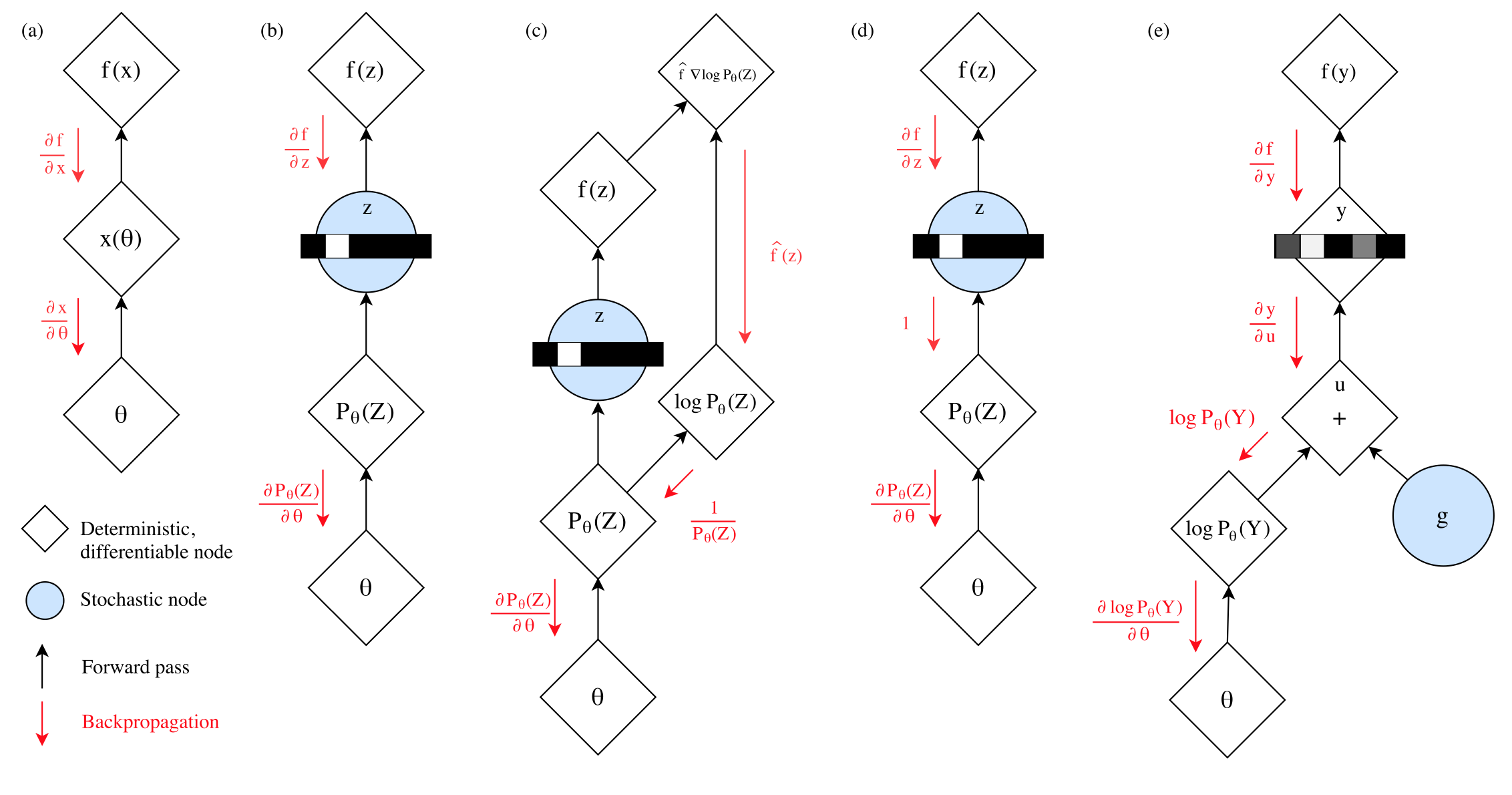
We can note that Gumbel-softmax is similar to the reparameterization trick used in Variational Autoencoders, in the sense that it shifts the stochastic part which is used in combination with the deterministic nodes to approximate the sample. The reparameterization trick cannot be applied here as the parameters are not adjusted for discrete distributions, but rather for a fixed set of distributions. Hence adjusting the parameters over multiple discrete distributions would not produce convergence neither coherent samples.
Kusner and Hernández-Lobato first employed it to create a language GAN POC with LSTM layers. Later came RelGAN, which also uses Gumbel-Softmax, and is built of a attention-based generator and a CNN-based discriminator. Its particularity is that it maps the input of the discriminator into several embedding sequences, which are passed independently to $d_\delta$. The several losses are averaged to get the final loss value. The authors expect each embedding sequence to represent different features of the input. Their results showed better BLEU metrics compared with other GAN baselines using RL to estimate gradients.
Finally, Chen et al. proposed an other approach with optimal transport. They replace the binary function of the discriminator by the Earth-Mover’s Distance (EMD) between the sentence features of real and synthetic data. However as computing the EDM is intractable in the case of neural language processing, they created an adaptation they called Feature-Mover’s Distance (FMD). On text generation and style transfer, their baseline show competitive results compared with other GAN-based sequential generative models such as SeqGAN (presented a few lines below).
Figure taken from Chen et al., the overall architecture of FM-GAN.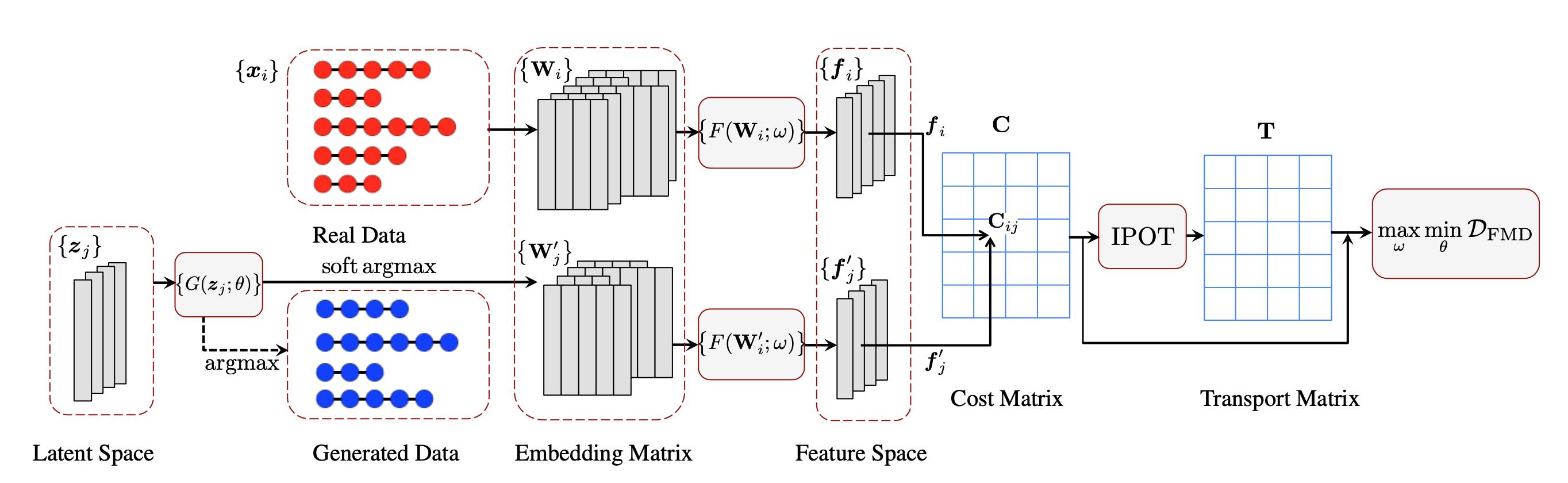
Reinforcement learning policy
In reinforcement learning, a policy is a strategy that an agent uses to realize its goals. The policy dictate its actions depending on its state and the environment. The policy is learned following a reward which is calculated by a cost function of its actions.
REINFORCE, also known as the score function estimator, transforms the integral into an expectation. It uses the log-derivative differentiation rule $\nabla_\theta\: p_\theta (x) = p_\theta (x) \nabla_\theta\: \mathrm{log}\: p_\theta (x)$.
We can then turn the gradient into an expectation:
$$ \begin{align} \begin{aligned} \nabla_\theta \mathbb{E}_{x \sim p_\theta (x)} &= \nabla_\theta \int f(x) p_\theta (x) dx \\ &= \int f(x) \nabla_\theta p_\theta (x) dx \\ &= \int f(x) p_\theta (x) \nabla_\theta \mathrm{log}\: p_\theta (x) dx \\ &= \mathbb{E}_{x \sim p_\theta (x)} [f(x) \nabla_\theta \mathrm{log}\: p_\theta (x)] \end{aligned} \end{align} $$
Now that the distribution under the expectation is known, we can estimate the expectation with Monte Carlo sampling. The key advantage of REINFORCE is that places no restriction on the nature of $f$, which does not have to be differentiable so that we can estimate the gradients of its expected value.
Due to the sampling, the gradients can easily suffer from high variance. Two solutions to reduces variances which can be applied here to stabilize training: control variates and importance sampling.
REINFORCE is used by SeqGAN. The generator is a reinforcement learning policy $G(y_t \lvert \mathbf{y}_{1:t-1})$ of generating a sequence. The discriminator provides the reward (the probability of being true data) $d_\delta (\mathbf{y})$ over the whole sequence. At step $t$, the state of $g_\theta$ is defined as the sequence of already predicted tokens $\mathbf{y}_{1:t-1}$. The discriminator $d_\delta$ estimates if the sequence $\mathbf{y}_{1:T}$ is real or generated, and its result is used as the reward to update the generator’s policy. The generator is made of LSTM layers, and the discriminator of convolutional layers. They experimented on text and symbolic generation. The reported results shows SeqGAN outperforming an MLE baseline, the same generator $g_\theta$ trained with teacher forcing, on BLEU and human metrics.
The same strategy is use with MolGAN and ScratchGAN, which generate respectively molecule graphs and text with results comparable to MLE baselines in term of quality.
RankGAN goes further by proposing a new training objective for the discriminator (called Ranker here). Given a collection of human-written and one generated sentences, it learns to rank them from the most human-like to the most fake. The learning objective of the generator is then to produce a sentence that is ranked higher by the ranker. These combined objective can be expressed as $\underset{\theta}{\mathrm{min}}\: \underset{\delta}{\mathrm{max}}\: \mathcal{L}(g_\theta, d_\delta) = \mathbb{E}_{x \sim p_d(\mathbf{x})} [\mathrm{log}\: d_\delta(x \lvert U, C^-)] + \mathbb{E}_{x \sim p_\theta(\mathbf{x})} [\mathrm{log} (1 - d_\delta(x \lvert U, C^+))]$ where $U$ is the reference ranking set and $C^-$ and $C^+$ are the comparison sets drawn respectively from fake sentences generated from $g_\delta$ and real data from $\mathcal{X}$. The score of a sentence $\mathbf{x}$ (either fake or real) coupled with a comparison set $\mathcal{C}$ is defined by:
$$d_\delta (\mathbf{x} \lvert \mathcal{U}, \mathcal{C}) = \mathbb{E}_{\mathbf{u}\ \sim\ \mathcal{U}} \left[\frac{\mathrm{exp} (\lambda \alpha(\mathbf{x} \lvert \mathbf{u}))}{\sum_{i=1}^{\lvert \mathcal{C} \lvert} \mathrm{exp}(\lambda \alpha(\mathcal{C}_i \lvert \mathbf{u}))}\right]$$
where $\alpha$ is the cosine similarity function. The ranking training objective learns the discriminator to not only distinguish fake for real data, but emphasizes on the learning of the underlying features comprised within the real data distribution in a kind of contrastive way.
Figure taken from RankGAN paper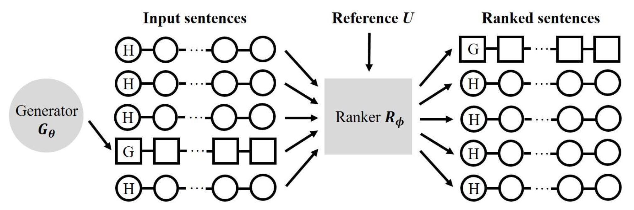
Note that some other low variance gradient estimator exist and can also be used in the case of GAN, such as Rebar or GO Gradient / GO Hessian.
Chunked auto-regressive generation GAN
CARGAN employs a kind of hybrid generation method, mixing autoregressive and non autoregressive, for conditional waveform synthesis. The generation can be formulated as follow: $g_\theta (\mathbf{y}, \mathbf{x}) = \prod_{t=i}^{T} g_\theta(\mathbf{x}_{t-k:t} \lvert \mathbf{x}_{1:t-k})$ where $i \in {k,2k,…,T }$. The model thus has predicts chunks of sequence of $k$ length, one after an other conditioned on the previous ones. This method is notably used by WaveRNN or WaveFlow, and is particularly well suited for the audio modality due its continuous but discretized nature, with a time dimension along which one can desire to extend the content. I am not sure that this technique would give results comparable with MLE models if applied to text, I have not seen something similar yet.
Issues with discrete GANs
A sequence of discrete elements is built of elements all dependant from each other. Hence sampling independently each element from a multivariate distribution is a very hazardous task. A token $y_i$ sampled first (with a high probability) could have no sense with another token $y_j$ is sampled (with a potentially high probability too). Hence we can doubt the capacity of a neural network to predict in a single step a sequence of discrete elements with coherent meaning. The nature of discrete data induces that a wide variety of plausible solutions close to the real data distribution $\mathcal{X}$ exist for most language modeling tasks. Hence even with the presented solution, discrete GANs are actually handling a hard and unpredictable task.
The conclusion is that language GANs still fall behind pure MLE-based models. Language GANs Falling Short empirically shows that discrete GANs tends to be more prone to mode collapse, and produce less diverse output. This is kind of expected, as the generator is trained to produce a multivariate distribution to fool a discriminator. We can very likely expect the model to learn a set of plausible examples and easily falling into mode collapse.
The paper also criticizes the fact that most language GANs introduced so far mostly focused on the quality of the results only. They claim that the difficulties to train a discrete GAN are not worth, and appear to be a larger problem than the exposure bias that this kind of model is trying to solve in the first place.
Alternative training objective
In 2020, Welleck et al. introduced unlikelihood training. They aim to tackle the exposure bias by altering the traditional teacher forcing training objective to reduce the probability of previous tokens.
Given a set of candidate tokens $\mathcal{C}$, the “unlikelihood” loss is defined as:
$$\mathcal{L}_{UL}(p_\theta (\cdot\: \lvert\: \mathbf{x}_{<t}),\: \mathcal{C}) = - \sum_{c\: \in\: \mathcal{C}} \mathrm{log}(1 - p_\theta (c\: \lvert\: \mathbf{x}_{<t}))$$
And during training the global loss is:
$$\mathcal{L}(p_\theta(\cdot\: \lvert\: \mathbf{x}_{<t})) = -\alpha\: \mathcal{L}_{UL}(p_\theta (\cdot\: \lvert\: \mathbf{x}_{<t}), \mathcal{C}) - \mathrm{log}(x_t \lvert \mathbf{x}_{<t})$$
The model will intuitively updates its parameters towards lower probabilities for tokens within $\mathcal{C}$. And the $\alpha$ constant controls how the unlikelihood loss contributes to the model’s training. By setting $\mathcal{C}$ as the previous tokens (${ x_1, …, x_{t-1} }$), the authors show that this technique helps the model to predict less repeated tokens when used autoregressively. Moreover, frequent tokens are intuitively less likely to be predicted as they are likely to be present in the previous one already.
While this token-level penalty helps a language model to predict better results by itself, it is limited to the prefixes of sequences from the training set, and might be unsuited or useless for zero-shot tasks. The mismatch between training data and generated data remains if no training objective that operates on the overall generated results is used. This motivated the authors to also include a sequence-level unlikelihood objective.
Given a prefix $\mathbf{x}_{1:k}$, they propose to decode a continuation $\mathbf{x}_{k+1:N} \tilde p_\theta (\cdot \lvert \mathbf{x}_{1:k})$, construct per-step candidate sets ${ \mathcal{C}^{k+1}, …, \mathcal{C}^{N} }$, and use a per-step sequence-level loss as:
$$\mathcal{L}_{ULS}^t (p_\theta (\cdot\: \lvert\: \mathbf{x}_{<t}),\: \mathcal{C}^t) = - \sum_{c\: \in\: \mathcal{C}^t} \mathrm{log} (1 - p_\theta (c\: \lvert\: \mathbf{x}_{<t}))$$
Authors choose to penalize repeating n-grams in the continuation.
This sequence-level loss is used to fine-tune a pre-trained baseline. The authors reported that only 1500 updates substantially reduced degeneration.
Adversarial methods
Given the issues previously introduced, researchers worked on methods to go beyond the maximum likelihood training objective (and teacher forcing) of sequential models, while keeping low (or acceptable) variances. Those are not GANs in the sense that they do not train a generator depending on a loss computed with a discriminator, but rather trained both independently and use them in cooperation afterwards.
RML
One of the first effort is the Reward Augmented Maximum Likelihood (RML) framework. The authors proposed here to add an additional term $r( \mathbf{y} \lvert \mathbf{y}^{*} )$, to the training objective, where $\mathbf{y}$ is a true expected result and $\mathbf{y}^*$ a result generated from the model, to guide it toward more realistic results during inference. The objective as an expectation and the gradient are expressed as:
$$ \begin{align} \begin{aligned} \mathcal{L}_{RML}(\theta, \tau, \mathcal{D}) = \sum_{(\mathbf{x}, \mathbf{y} \in \mathcal{D})} \left\{ - \sum_{\mathbf{y} \in \mathcal{Y}} q(\mathcal{y} \lvert \mathcal{y}^* ; \tau) \mathrm{log} p_\theta (\mathbf{y} \lvert \mathbf{x}) \right\} \\ \nabla_\theta \mathcal{L}_{RML}(\theta, \tau) = \mathbb{E}_{p_\theta (\mathbf{y} \lvert \mathbf{x})} \left[ -\nabla_\theta \mathrm{log} p_\theta (\mathbf{y} \lvert \mathbf{x}) r(\mathbf{y} \lvert \mathbf{y}^*) \right] \end{aligned} \end{align} $$
Where $\tau$ controls the degree of regularization. This term can be based on any reward or metric such as BLEU. The training objective is equivalent to a RL one, but here we do not need to sample successively from the model and thus get a potentially very sparse gradient (given the high dimension of the associated space) with high variance. The results show naturally better BLEU metrics than their pure MLE counterparts on machine translation tasks, with a RNN model. The authors did not use this framework adversarially, but this could be done with $r$ as a feedback from a discriminator, as it will be achieve in future works.
Coupling autoregressive generation with Gibbs sampling
Su et al. proposed to couple a generator language model with a discriminator, and Gibbs sampling, in order to iteratively refine an input sentence until it satisfies some user-defined constraints. Gibbs sampling is a Monte Carlo Markov Chain (MCMC) sampling strategy that iteratively sample from a multivariate distribution $\mathbf{Y} \in \mathbb{R}^{L \times c}$ which would be to complex to sample from in one step. For $T$ steps, each element of the sequence is resampled $x_i \sim p_\theta (x_i \lvert \mathbf{x}_{\backslash i})$. As $\mathbf{x}$ is resampled, it becomes more natural following $p_\theta$.
The authors actually trained $K$ discriminators on $K$ constraints which return $d_k (c_k \lvert \mathbf{x})$, and $d(\mathbf{c} \lvert \mathbf{x}) = \prod_{k=1}^{K} d_k (c_k \lvert \mathbf{x})$. An input sentence is corrected multiple times in parallel by keeping the most likely tokens at each correction step, removing candidates for which $d(\mathbf{c} \lvert \mathbf{x}) < threshold$, and returning the candidate maximizing $d(\mathbf{c} \lvert \mathbf{x})$.
Discriminator guidance and MCTS
Holtzman et al. used learned discriminators, each specializing in a different aspect of human conversational communication, to train a RNN model to generate text.
DAS (Discriminative Adversarial Search) also inspired by adversarial training, trains a discriminator to tell apart generated text from human written text. It’s main goal is to reduce the exposure bias of traditional NLG methods. The discriminator predicts a label for each token instead of for the entire sequence. The discriminator logprob is added to the score to guide sampling toward the human-written style. This adversarial training allows to train several times the discriminator until it fails to detect machine learning results.
Figure taken from DAS: Overview of the DAS training procedure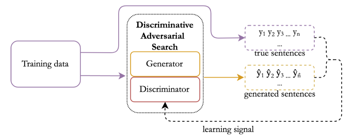
Scialom et al. further increases the link between generator and discriminator by introducing a discrete adversarial training framework: SelfGAN; and a cooperative generation decoding adapted from Monte Carlo Tree Seach (MTCS): Coopt-MCTS.
The SelfGAN framework can be expressed as following (note that we omitted the context from the original paper which corresponds to a seq2seq / encoder-decoder model architecture):
Input: Generator g, Discriminator d, cooperative decoding method c, training set X

for n epochs do
    for x in X do
        s_coop <-- c(x, g, d)
        g.train(input=x, target=s_coop)
        d.train(real=x, fake=s_coop)
The cooperative decoding uses the discriminator to steer the generator toward humans results. Used during the training stage as the expected target for the generator’s training, it allows to progressively improve both models at the same time.
Coopt-MCTS employs MCTS in order to progressively generate the results while maintaining its quality according to the discriminator. The root is $\mathbf{x}$, i.e. the input token sequence to extend, to which is associated a score $s_0 = d_\delta (\mathbf{x})$. The child of a node is the next token to be selected. The objective is to find the path (sequence $\mathbf{y}$ which extends $\mathbf{x}$) for which $d_\delta (\mathbf{y})$ (or other part or subparts, including $\mathbf{x}$) is minimized, without exploring the whole tree, for optimization and complexity reasons.
- Selection: children nodes (tokens) are iteratively selected. The probability $g_\theta (\mathbf{x}_t )$ for the next token $x_{t+1}$ are used to this end, associated with the PUCT algorithm. Nucleus sampling is applied to reduce the set of possible tokens and discard those with low probabilities: $P(x_i) = s_i + c_{puct} g_\theta (x_i \lvert \mathbf{x}_{1:i-1}) \frac{\sqrt{\sum_{b}N(\mathbf{x}_{1:i-1}, b)}}{1 + N(\mathbf{x}_{1:i-1}, x_i)}$ where $c_{puct}$ is a constant, $N(\mathbf{x}, w)$ is the number of times $w$ was selected for the sequence $\mathbf{x}$, and $s$ is the score of the node given by the discriminator as $s_i = d_\delta (\mathbf{x}_{1:i})$.
- Expansion: if the children is not in the final state ($T$), extend it with $g_\theta$ and nucleus sampling.
- Simulation: when a child reaches the final state ($T$), we use the discriminator to evaluate it $d_\delta (\mathbf{y})$.
- Backpropagation: when a node becomes terminal (End of Sequence token or maximum length), the scores of its parent nodes back to the root are updated, as $s_i = \mathrm{max}(s_i, s_0)$
These steps are executed for a maximum number of steps, after which the next token of the root is selected by taking the one with the most visits. All is repeated to predict token by token the continuation of the sequence, until reaching a special token End Of Sentence, or the maximum length.
Note that the discriminator becomes more accurate as the sequence length it judges grows. If a long sequence is overall judged human, all its subsequences could also be considered human. And a sequence could be judged fake although its beginning could be judged human. The main advantage of Coopt-MCTS is that 1) the discriminator is used on sequence of relatively large sizes, which is how it should be used; 2) it allows to accurately explore nodes and chose the one considered humans, resulting in an overall good quality result.
Lamprier et al. further improve the cooperative generator-discriminator framework by introducing a partition function which regularizes the calculation of gradients while assuring convergence of both the generator and discriminator networks.
One of the main issues of cooperative frameworks so far was that their convergence was not proved and assured. For most of these works, the model distribution is updated by maximizing the likelihood between the probabilities $g_\theta (\mathbf{x})$ and a target distribution which is the result of some cooperation decoding $q = \mathrm{c}(p_\theta, d_\delta)$. We can express this is minimizing $\mathrm{KL}(q \lvert\lvert p_\theta)$.
But if we consider $q \triangleq \mathrm{c}(p_\theta, d_\delta) \propto exp(d_\delta)$ where this distribution is only proportional to the outputs of the discriminator, and a step where the generator is optimal (i.e. $p_\theta \approx p_d$). In the next step, the optimal discriminator yields $d_\delta(\mathbf{x})=0.5\; \forall\; \mathbf{x} \in \mathcal{X}$, thus optimizing the generator with $q \propto exp(d_\delta)$ will make it diverge from the optimal $p_d$. While being extreme, this examples illustrate the instabilities of convergence this recent family of model can suffer from.
Instead, the authors proposed to set $q \propto p_\theta ,d_\delta$, which theoretically guaranties convergence: if the generator and discriminator have enough parameters, as we successively train them, $p_\theta \rightarrow p_d$ and $d_\delta(\mathbf{x}) \rightarrow 0.5\; \forall\; \mathbf{x} \in \mathcal{X}$.
Moreover, if both parts of the discriminator are sufficiently trained (its mean is superior to 0.5), we have $\Delta \triangleq \mathrm{KL}(p_d \lvert\lvert p_\theta) - \mathrm{KL}(p_d \lvert\lvert p_\theta) \leq \mathrm{log}(\eta^{-1} - 1) > 0,; \eta \in \left[ 0.5; 1 \right]$, meaning $q \propto p_\theta ,d_\delta$ is a useful target to move toward.
The gradients of our previous objective $\mathrm{KL}(q \lvert\lvert p_\theta)$ can be rewritten with importance sampling as:
$$ \begin{align} \begin{aligned} \nabla_{p_\theta}\: \mathrm{KL}(q \lvert\lvert p_\theta) &= -\mathbb{E}_{\mathbf{x} \sim q(\mathbf{x})} \left[ \nabla\: \mathrm{log}\: p_\theta(\mathbf{y}) \right] \\ &= -\mathbb{E}_{\mathbf{x} \sim p_\theta(\mathbf{x})} \left[ \frac{q(\mathbf{x})}{p_\theta(\mathbf{x})} \nabla\: \mathrm{log}\: p_\theta(\mathbf{x}) \right] \\ &= - \frac{1}{Z}\: \mathbb{E}_{\mathbf{x} \sim p_\theta} \left[ d_\delta(\mathbf{x}) \nabla\: \mathrm{log}\: p_\theta(\mathbf{x}) \right]\\ Z &= \sum_{x \in \mathcal{X}} p_\theta(\mathbf{x}) d_\delta(\mathbf{x}) \end{aligned} \end{align} $$
$Z$ is the partition function of the discriminator and acts as a regularization of the gradient calculation. It can be written as an expectation $\mathbb{E}_{\mathbf{y} \sim p_\theta(\mathbf{y})} \left[ d_\delta(\mathbf{y}) \right]$, where it is clear that $Z$ is maximized when samples from $p_\theta$ are likely to be close to $p_d$. This term naturally avoid the explosion of gradient and the use of complex and tedious learning rate scheduler, which are often required with other discrete GAN settings.
Chaffin et al. empirically showed that an unidirectional transformer (causal attention mask) achieves results comparable to a bidirectional one (no attention mask), while being much more efficient. At inference, the previous hidden states can be reused as they do not need to be recomputed considering the tokens lastly sampled.
Aligning LMs with human preferences
Generating coherent and context-dependent text is often very hard, and its quality/prompt-matching is hard to measure. Most LMs are autoregressive Transformers trained with a teacher forcing (i.e. next token prediction) objective, that do not capture the subjective human preferences. To address bridge this gap, Reinforcement Learning with Human Feedback (RLHF) has become a very popular technique in the last few years, especially for industrial actors who want to put LMs in real-life conditions (such as InstructGPT, then ChatGPT, Gopher).
RLHF: Reinforcement Learning with Human Feedback
RLHF uses reinforcement learning to optimize a LM with human feedback, in order for it to generate more aligned results. In traditional RL, an agent learns by interacting with an environment, receiving feedback in the form of rewards or penalties based on its actions. RL algorithms, such as Q-learning or policy gradients, optimize the agent’s behavior to maximize cumulative rewards over time. In RLHF, humans are involved in the learning process by providing additional feedback to the reward model / preference model. This feedback can take various forms, such as explicit rewards, preference rankings, demonstrations, or critiques. The reward model takes in a sequence of text, and outputs a scalar reward calibrated with human preferences (feedback). It can be an other LM trained on the human feedback data.
To get human feedback data, human annotators are asked to assess text generated from the LM to finetune. This is mostly done by asking them to rank several sentences generated by different models. This allows to get a much better regularized dataset of feedback than asking humans to give scalars feedbacks, as their perceptions are subjective and greatly vary. This approach coupled with an Elo ranking system, allows to have more uniform relative rankings distributions to train the model with.
Training a model with RL is usually done with a policy algorithm, such as Proximal Policy Optimization (PPO). In our case, the policy is our generative LM, the environment (or action space) is the set of all tokens of the vocabulary, the observation is the possible input token sequences. The reward function is the reward / preference model (RM). The RM takes in a prompt and a generated answer, and outputs a score. It is trained with pairs of a winning and a losing answers generated by two different LMs, to minimize the expected loss $\mathbb{E} \left[ \log (\sigma (\mathbf{s}_w - \mathbf{s}_l)) \right]$ ($\mathbf{s}_w$ and $\mathbf{s}_l$ are the scores for the winning and losing answers respectively).
Once trained, the RM is used to train the LM. In practice, the loss is combined with a constraint on policy shift. The constraint is here to assure that the model do not stray to much compare to its original version. The reason is that there are many possible responses to a prompt, that the RM has not been trained on. Moving too much the parameters might satisfy the RM, but would limit the diversity and even generate bad aswers that still yield high rewards.
In practice, only a few parameters are updated during finetuning, as optimizing the whole model is often quite expensive in compute resources (LoRA, Sparrow). One of the biggest challenge of RLHF was actually to figure out how to adapt it to finetune LLMs.
Overview of the RLHF process.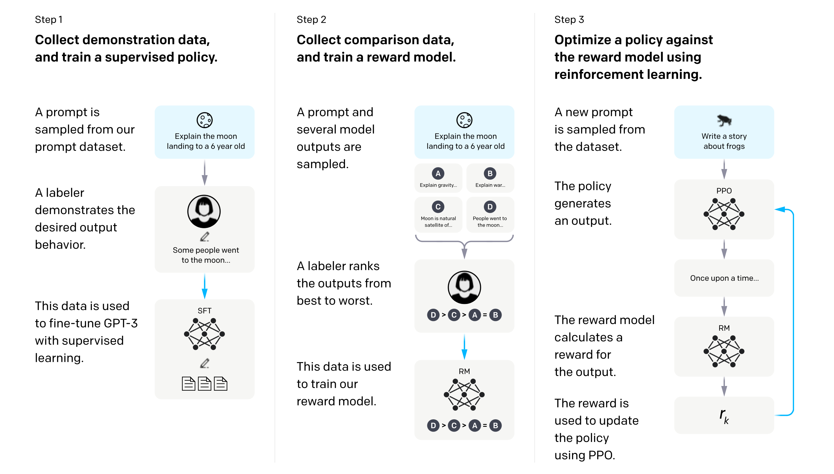
RLHF can finetune a LM towards more human, coherent and less toxic results. The overall process is relatively simple and can be automated. It can be iteravely performed to further improve a model’s capacilities (a process called Iterated Online RLHF). However, getting human feedbacks is not an easy task, and in most cases becomes quite expensive (as often done through crowdsourcing platforms such as MTurk). That is one of the reasons OpenAI released ChatGPT free to the public, as it allows them to get free feedbacks and further improve the backbone model.
DPO: Direct Preference Optimization
We have seen so far how human preferences have been used with RL and PPO to finetune LMs. What we haven’t tell is that PPO is a complex procedure that is often unstable in practice.
Rafailov et al. introduced DPO (Direct Preference Optimization), an alternative human preference alignment techniques that does not require to train a reward model, but directly optimize the LM with respect to the preference data. There is actually no RL involved, and the LM itself can be seen as the policy.
DPO is stable, lightweight and much more easy to implement and perform. Classifier reward models often only reach ~70% accuracy on training set and ~60% accuracy on evaluation set, whereas DPO rapidly reaches 100% training accuracy and ~80% accuracy on the evaluation set.
Enhancing LMs with external sources
When used during inference as is, LMs make predictions based on the correlations of token occurrences in the data they are trained with. For LLMs, the training data is often scrapped from contents from the internet: Wikipedia, press media, social media and public forums. This results in generations that: 1) can be biased towards the training data, for its content as well its form or style; 2) the model is unaware of any news of the current world dating after the training data.
Leveraging external (new) data could allow LMs to make more accurate predictions, or even make predictions they does not have the capabilities to make without it. This is the motivation of Retrieval-Augmented Generation (RAG).
RAG: Retrieval-Augmented Generation
The general idea of RAG is to leverage a database of embedding vectors of external data to provide more information to a LM. The term was introduced by Lewis et al. in 2020. In practise, a sentence embedding is extracted from a user prompt with an embedding model. The prompt-embedding is compared to those of an embedding database, with a search library such as Faiss. The data (text) of the matching embeddings is retrieved and passed to the LMs along with the original prompt, to generate an answer, potentially citing sources from the embedding database.
Overview of RAG.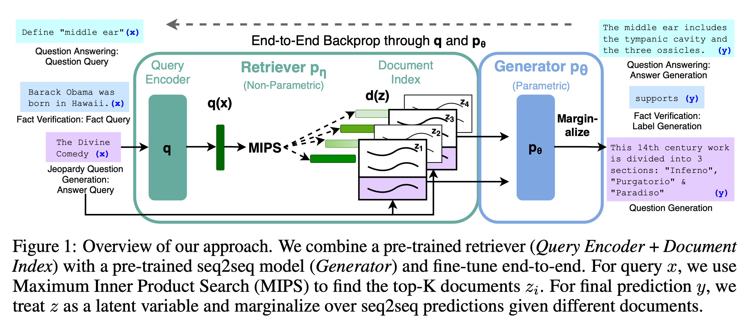
The embedding database is continuously updated with new data, the LM then stays up to date.
Despite this relatively simple presentation, RAG is a complex method that raises a lot of challenges to implement. Hopefully, open-source frameworks such asLangChain or RAGatouille allows to easily build a RAG pipeline.
Contrastive learning for text generation
CoNT
CoNT, for Contrastive Neural Text, addresses the exposure bias with contrastive learning. It is a framework that can be used to train and infer from any language model.
Instead of naively applying contrastive loss terms as done with other modalities, CoNT:
- Uses generated samples to set the contrastive loss;
- Uses a N-pair loss which includes sequence-level scores of all pairs;
- Directly incorporates the learned sequence similarity score from the distance function into the inference stage.
Overview of the CoNT framework. Figure taken from the original paper.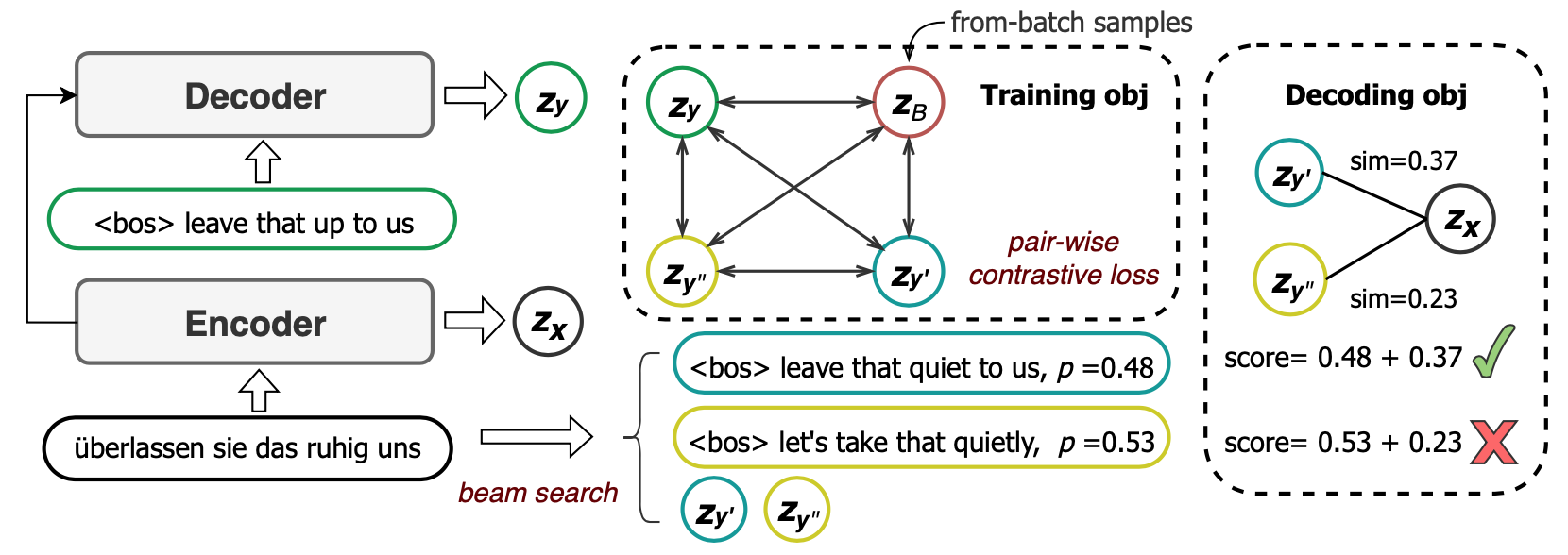
Common contrastive loss terms are built from samples within a batch. Whereas it satisfies very well the overall training objective, it does not address the exposure bias issue. Using generated samples to build the contrastive loss allows to expose the model to its mistakes. The authors use beam search to generate them, and also note that a warm-up stage where the model is only trained with a pure NLL loss is recommended so that the generated samples have a sufficient quality.
Common contrastive loss also treat all negative samples equally, meaning that the relative difference between real and generated samples is ignore. To mitigate this, CoNT employs a pair-wise margin loss: 1) all generated samples are ranked with an oracle function $o(\cdot, \textbf{y})$ which computes a sequence-level score according to the real sample $\mathbf{y}$. The overall contrastive is formulated as:
$$\mathcal{L}_{N-pairs} = \sum_{(\mathbf{y}^-, \mathbf{y}^+) \in \mathcal{P}} \mathcal{L}(\mathbf{y}^-, \mathbf{y}^+) = \sum_{(\mathbf{y}^-, \mathbf{y}^+) \in \mathcal{P}} \mathrm{max} \left( 0, \mathrm{cos}(\mathbf{z}_{\mathbf{x}}, \mathbf{z}_{\mathbf{y}^-}) - \mathrm{cos}(\mathbf{z}_{\mathbf{x}}, \mathbf{z}_{\mathbf{y}^+}) + \gamma \right)$$
$\mathcal{P}$ is a set of pairs of samples, made of real and generated samples. The latter are classified $\mathbf{y}^-$ or $\mathbf{y}^+$ depending on their ranks. $\mathrm{cos}(\cdot, \cdot)$ is the cosine similarity function, $\mathbf{z}_{\mathbf{i}}$ is the hidden representation of the input sequence $\mathbf{i}$, and $\mathbf{x}$ and $\mathbf{y}$ is the input sequence. During inference, this learned similarity score is included to steer the predictions towards results closer to the data distribution.
SimCTG
SimCTG introduces a contrastive approach based on the similarity of the embeddings of tokens. The authors show that, with a model trained with a pure MLE training objective, the cosine similarities between the embeddings of the successively predicted tokens are relatively high. This is mostly explained by the anisotropic embedding distributions that most LM learn, especially generative ones (Ethayarajh, Cai et al). This is counterintuitive for generative tasks, where we expect a model to yield high probabilities to tokens that are both coherent considering the past context, and informative (as opposite to degenerating, topic drifting or repetition). They thus introduced SimCTG, as a contrastive loss term, defined as:
$$\mathcal{L}_{CL} = \frac{1}{\lvert \mathrm{x} \lvert \times (\lvert \mathrm{x} \lvert - 1)} \sum_{i=1}^{\lvert \mathrm{x} \lvert} \sum_{j=1, j \neq i}^{\lvert \mathrm{x} \lvert} \mathrm{max} { 0, \phi - s(\mathbf{h}_{x_{i}}, \mathbf{h}_{x_{i}}) + s(\mathbf{h}_{x_{i}}, \mathbf{h}_{x_{j}}) }$$
In the equation above, $\phi \in [-1, 1]$ is a margin, $s(\cdot)$ is the cosine similarity function, $\mathbf{h}_{x_i}$ is the embedding of $x_i$, from the input sequence $\mathbf{x}$.
During training, the overall loss is set as $\mathcal{L} = \mathcal{L}_{MLE} + \mathcal{L}_{CL}$. This insure that the model still learns with teacher forcing to predict the next tokens according to the past ones, while making sure that it produces discriminative and isotropic embedding representations.
The authors also introduced a contrastive decoding method, defined as:
$$x_t = \underset{v \in \mathcal{V}^{(k)}}{\mathrm{arg max}} { (1-\alpha) \times p_\theta(v \lvert \mathrm{x}_{<t}) - \alpha \times (\mathrm{max} { s(\mathbf{h}_v, \mathbf{h}_{x_j}) : 1 \leq j \leq t-1 })}$$
$\mathcal{V}^{(k)}$ is the set of top-k predictions from $p_\theta(\cdot \lvert x<t)$, $\alpha$ balances the two components. The first is the model’s probability distribution and represents its confidence. The second measures how discriminative of candidate $v$ with respect to the previous context $\mathbf{x}_{<t}$, represents the degeneration penalty. A larger degeneration penalty of $v$ means it is more similar to the context, therefore more likely leading to model degeneration.
SimCTG associated with the contrastive decoding was shown to outperforms most common decoding methods such as beam search, top-k and nucleus.
Contrastive decoding
Contrastive Decoding (CD) is another decoding strategy, based on two LM: a small “amateur” LM, and bigger “expert” LM. Smaller LM tend to be more prone to exposure bias failures, and that their probability distributions can be used as a signal to be sent to a larger one to increase the quality of generated results. CD produces higher quality text than decoding from the larger LM alone, and can be used with any LM.
Schema of contrastive decoding. Figure taken from the original paper.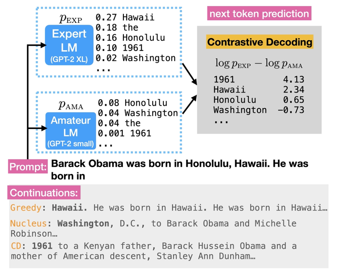
LookBack decoding
Similarly to Controastive Decoding, Look-back leverage the previous context to steer the next token selection. The authors show that the Kullback-Leibler (KL) divergence between the probability distributions generated by a LM between a step $t$ and the previous ones tends to stay low for repetitive tokens, or tokens with similar semantics. They also show that the KL divergence between the distribution of step $t$ and steps of a prefix can easily increase as the topic drifts over the generated tokens.
To alleviate these issues, they propose to “trigger” a different sampling behavior when the minimum $KL_{min}^t$ (defined below), the minimum KL divergence between the probability distribution of the current step $t$ and the distributions of the steps $j$ to $t-1$.
$$KL_{min}^t = \underset{1 \leq j \leq t-1}{min} KL (p(x_{\leq t}) || p(x_{\leq j}))$$
When $KL_{min}^t$ is lower to a defined threshold α, the next token is sampled from the top-k most probable ones, otherwise the most probable one is selected (greedy). $KL_{min}^t$ can also be measured between the current step and the steps of a prefix, between the steps $t_1$ to $t_2$, in order to reduce topic drift.
Results with GPT2-XL and OPT-6.7B on WikiText-103 and WritingPrompts showed Look-back outperforming other common decoding methods, on MAUVE and coherence metrics as well as human evaluations. The authors also highlight the limitations of the approach: it can penalize tokens with low KL divergences, that would be desired repetitions; it produce more bi-gram repetitions, at least when $KL_{min}^t$ is measured on a prefix.
NPM: NonParametric Masked Language Model
NPM addresses a major limitation that is often not stated in language modeling: the bottleneck of reliying on a softmax distribution over a finite vocabulary to perform LM tasks, such as classification or information retrieval. LMs usually have difficulties to have good accuracies when dealing with rare words or use-cases, and the softmax approach also limits their adaptation to new domains and tasks.
Instead of making predictions over the usual parametric vocabulary distribution, NPM does over a non-parametric distribution of embedded phrases from a reference corpus. The idea consists to map all the phrases from the reference coprus into a continuous vector space using an encoder LM, and infere from the same encoder by replacing [MASK] tokens in the input by the nearest phrase from the corpus. NPM can be trained with phrase-level contrastive learning objective (hence why it is in this section), with masked spans of input sentences and in-batch positives and negatives.
Results show that NPM is significantly more parameter-efficient, outperforming up to 500x larger parametric models and up to 37x larger retrieve-and-generate models.
Although the out-of-the-box application of this concept to NLG is not clear, it still challenges the common autoregressive prediction for simple information retrieval, and I thought it has its place here as it could serve as reference and give some inspiration for new ideas.
Gradient-based generation and diffusion models
Diffusion models have emerged as the goto solution for image generation in hte last years. TLDR, they are a category of model trained to remove noise from a latent distribution. During inference they are iteratively used to generate content from noise, and can even be conditioned for controllable generation. In other words, the generation is guided by the gradients of the denoising process. However, they work on joint (continuous) distributions, are hence non-autoregressive, so their application to natural language or other discrete modalities has not been straightforward. Here is a great blogpost intrdocing in details diffusion models.
As for continuous modalities, text diffusion aims to gradually denoise a categorical distribution. The starting noise can be either discrete (token, $\mathbf{x}_T \in \mathbb{R}^{L}$) or continuous (embeddings, $\mathbf{X}_T \in \mathbb{R}^{L \times d}$), while the network is a LM (e.g. Transformer). The overall process can be expressed as:
$$p_\theta (\mathbf{X}_T \lvert c) = \prod_{t=0}^{T-1} \prod_{i=1}^{n} p_\theta (\mathbf{x}_i \lvert \mathbf{X}_{t+1}, c, t)$$
The diffusion process for discrete state spaces has been first introduced by Solh-Dickstein et al. who formulated a diffusion process over binary random variables, before being generalized and adapted for different usages.
COLD decoding
COLD decoding is one the first attempts to leverage gradient to guide text generation. Even if the paper does not state the use of diffusion, the backbone, Langevin dynamics, is the same.
COLD decoding generates text by sampling from the distribution of an EBM function obtained with iterative Langevin dynamics. The continuous sample is discretized with top-k sampling into fluent text.
Figure taken from the COLD Decoding paper: Overview of the COLD decoding procedure.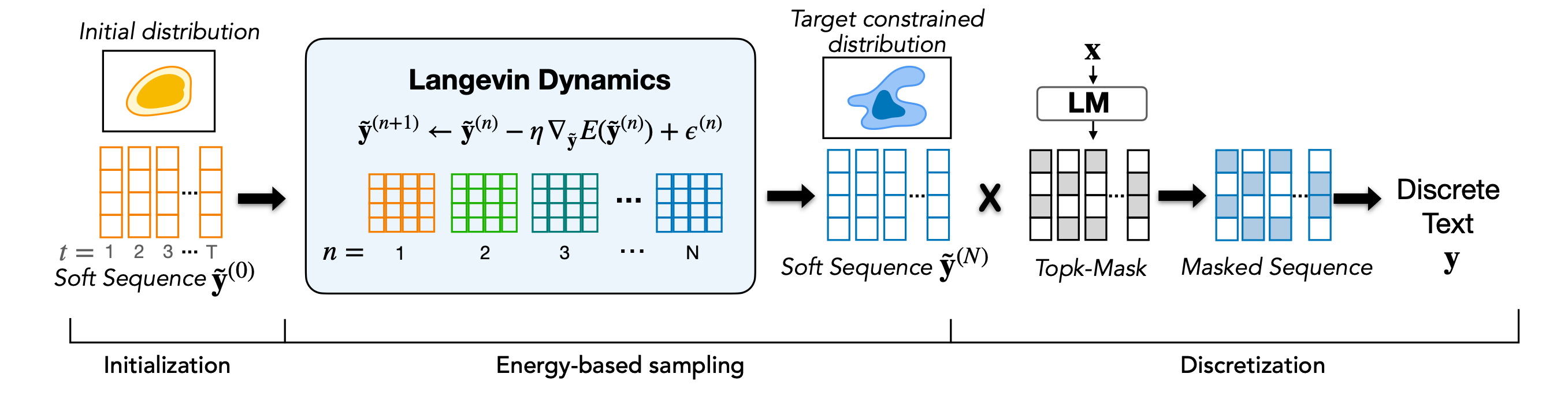
In the figure above, the soft sequence $\tilde{\mathbf{Y}}$ is drawn from constraint tokens is iteratively refined toward the target constrained distribution after $N$ steps, given an energy function $E(\tilde{\mathbf{Y}}) = \sum_{i} \lambda_i f_i(\tilde{\mathbf{Y}})$.
An appealing advantage of COLD decoding is it can be associated to any sequential model, and allow to dynamically filter the output tokens according to constraints, even high level or structural one which are known to be hard to satisfy.
Argmax Flows and Multinomial Diffusion
Hoogeboom et al. introduced a method to perform diffusion on categorical random variables, by using $\mathrm{arg max}$ function to iteratively “discretize” the distributions over each steps. The input tokens are represented as one-hot vectors, while the output distributions can be rounded with Gumbel and thresolding. The whole diffusion is hence “multinomial”. The authors experimented with working results on image segmentation and text generation, with results of lower coherence than AR for the latter. D3PMs is a generalization of this previous formulation, by corrupting the input with uniform transition probabilities based on nearest neighbors in embedding space. This allows to add another “depency” layer between each distributions, following the discrete nature of the process. During inference, the model starts from [MASK] tokens and iteratively substitutes them with word tokens until the desired text is generated. The model achieves coherent results on character-level text generation, ans is able to scale to large vocabularies.
Performing diffusion on continuous variables
Diffusion-LM perform diffusion on continuous variables. The model iteratively denoises a sequence of Gaussian vectors into word embeddings. As these intermediate variables are continuous, the gradient-based updates are quite straightforward to perform. In the backward process, the model empirically fails to generate $\mathbf{X}_0$ embeddings that commit to the actual learned embeddings. $\mathbf{X}_0$ are then “converted” to tokens with a “rounding” process $p_\theta (\mathbf{w} \lvert \mathbf{X}_0) = \prod_{i=0}^{L} p_\theta (w_i \lvert \mathbf{x}_{0,i})$ where $p_\theta (w_i \lvert \mathbf{x}_{0,i})$ is a softmax distribution. During inference, the authors apply Minimum Bayes Risk to the decoded embeddings in order to sample a final sequence of tokens minimizing the expected risk under a loss function (parametrized with a metric such as BLEU). They however do not share details on the number of candidates $\mathcal{S}$ and the loss used in their experiments. The model can be also controlled with classifier guidance for controllable generation. Finally, the decoding speed of the model is still lower than for AR counterparts. The authors note: “Decoding Diffusion-LM for 200 steps is still 7x slower than decoding autoregressive LMs.”.
Overview of the Diffusion-LM forward and backward passes. Figure taken from the Diffusion-LM paper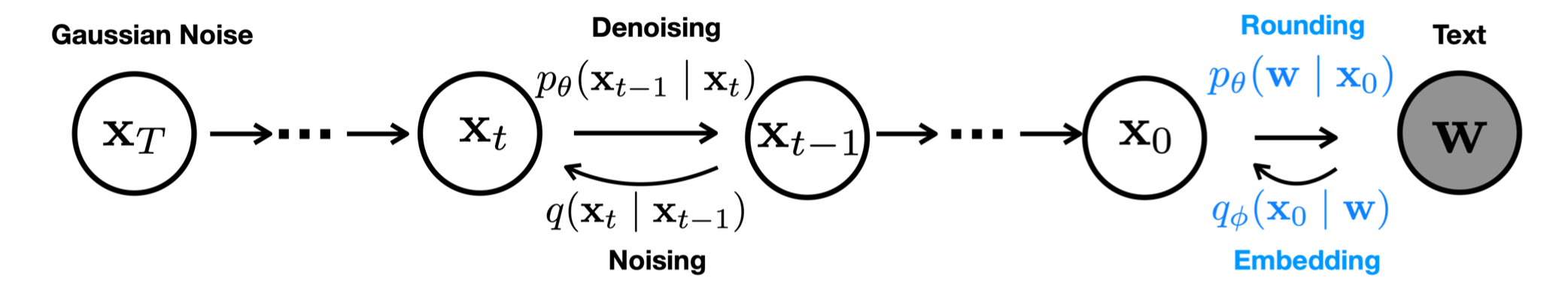
Chen et al. relied on the same process, but designed a different noising, they called soft-masking, which apply different scales of noise to the embeddings depending on their importance, measured as a combination of word relevancy and entropy (as an estimation to the level of information).
DiffuSeq uses classifier-free guidance and show that it further improves the prompt-result alignment.
GENIE is an seq2seq model, with a diffusion-based decoder. The decoder is a transformer, which iteratively denoises gaussian noise while being conditionned on the hidden states produced by the encoder with cross-attention. One of the main novelty of the paper is the continuous paragraph denoise (CPD) training technique. During the training, a randomly selected portion $\mathbf{p}$ of the input sequence is masked with special MASK tokens. The masked input is fed to the encoder, and the decoder is trained with $\mathbf{p}$. The decoder hence is learns to generate the masked paragraph.
GENIE was evaluated on four text generation benchmarks, XSum, CNN/DailyMail, Gigaword and CommonGen, achieving competiting results with AR transformer counterparts on BLEU and ROUGE metrics.
However, the authors didn’t justified the choice of randomnly select $\mathbf{p}$. We can wonder what the effect would be if we instead segment the text data by paragraphs or (groups of) sentences.
CodeFusion is a more elaborated diffusion model for the text-to-code task. The model architecture consists of three main parts: an encoder processing the text query into continuous hidden states, a denoiser diffusion model which iteratively denoises gaussian noise into embeddings conditionned on the hidden states, and a decoder mapping the denoiser’s output into descrete tokens. The denoiser is trained with the continuous paragraph denoise (CPD) techniques from the GENIE paper introduced above.
Overview of the CodeFusion model architecture. Figure taken from the CodeFusion paper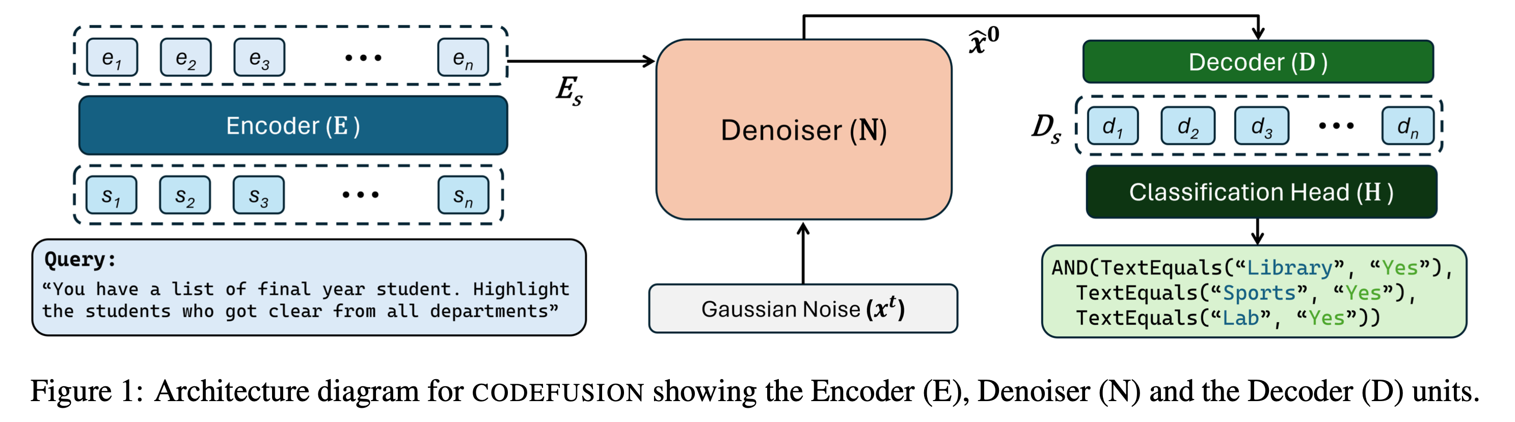
Code generation is a task especially prone to the exposure bias’s effects. As the combinations of tokens can represent compex logic tasks, it is common that some lines of code can be generated with inconsistencies with the previous ones. Here, the results of the paper show CodeFusion (70M parameters) outperforming larger models (among which ChatGPT and GPT-3) on several programming languaegs (Python, Bash, CF Rule) (top-1, top-3, top-5 predictions). However, no numbers have been shared on its time and latency during inference.
“Autoregressive” diffusion models
So far, we have explored works applying the “vanilla” diffusion process to sequential data, meaning generating series of tokens simultaneously, similarly to the pixels of an image. While these applications have been showned to work with models able to generate text, their inference process do not consider the sequential and ordered nature of natural language. This disparity is worth to be looked in, as the earliest elements of a sequence naturally influence what the following one are. Of course the advantage of diffusion models over AR models is their ability to adjust elements of the sequence that are not the last one, however treating every token position equally can be seen as counterintuitive considering their sequential dependency.
“Autoregressive Diffusion Models” (ARDM) is a first atempt to make an autoregressive discrete diffusion model. ARDM is order agnostic, meaning able to generate tokens in any order. In ARDM, a sequence of variables is autoregressively predicted in an order $\mathbf{\sigma} \in \mathbb{N}^L$ sampled from the set of possible permutations of $L$ positions. The process allows to generate these variables in parallel during inference. The authors experimented with the text8 dataset, reporting lower NLL losses (and no other metrics) than those of order agnostic counterparts. Indeed, and the authors highlight it, the approach is not competitive with common autoregressive approaches. This could be attributed partly to a big limitation of the randomly sampled order: when a defined number of tokens $m$ separating the already generated positions $n_1$ and $n_2$ do not satisfy $n_1 + n_2 = m$, we can expect the model to predict incoherent results. Experiments with continuous modalities, namely images and audio, showed good results for compression and upscaling tasks, for which the order of the variables plays a lesser important role than for natural language.
Generation of variables with ARDM. Figure taken from the Autoregressive Diffusion Models paper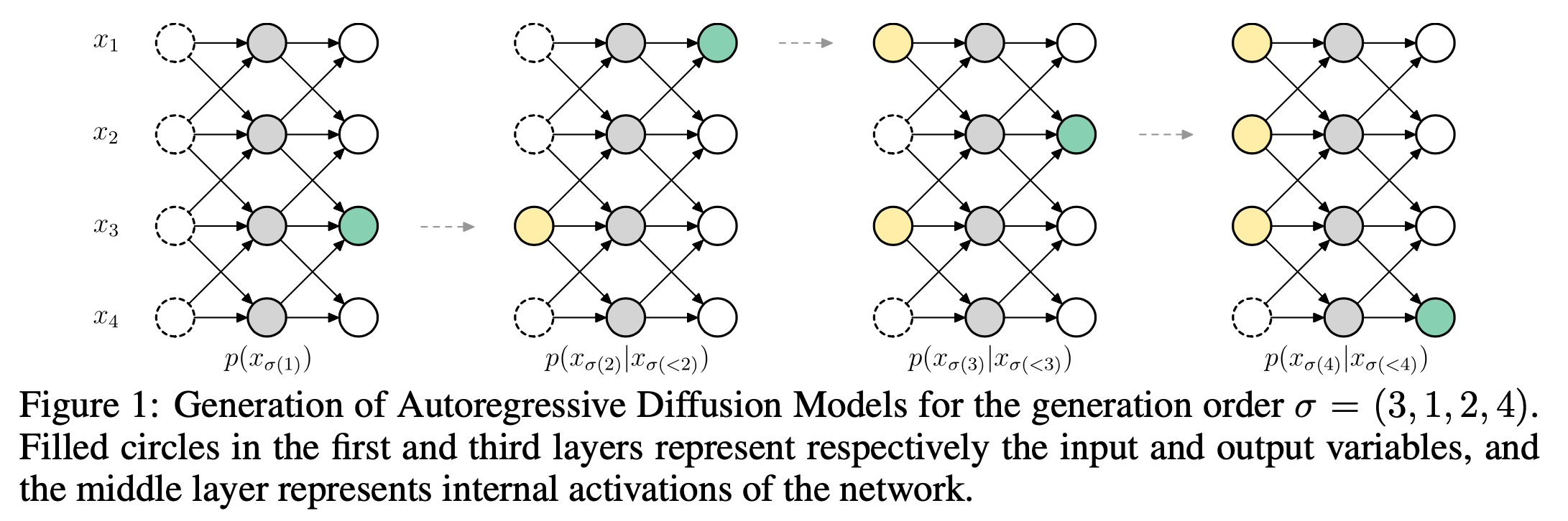
SSD-LM is a semi-autoregressive approach, which simply consists in iteratively generating successive chuncks of tokens, with biderectional context within each chunk being generated. The model works on the simplex space of the vocabulary, i.e. probability distributions in input and output instead of learned embeddings. The tokens are converted to “almost-one-hot” vectors $\mathbf{x}_i = {k \mathrm{if} j=i, -k \mathrm{otherwise}}_{j=0}^{\lvert \mathcal{V} \lvert}$ ($k$ is an hyperparameter) intended to mimic the logits (performing softmax on $\mathbf{x}_i$ results in an almost one-hot vector). It allows to avoid having to map the generated embeddings to discrete tokens after the final diffusion step. However, the authors added a projection operation to the denoised logits for each diffusion step. No experiments have been conducted without projection, i.e. denoising the raw output logits from the previous step. A drawback of working with logits on the vocabulary simplex is that the model will not take advantage of the learned embedding capacilities of LMs, especially knowing the pre-trained models are now abundant. The pros and cons of both approaches need to be further investigated. The authors achieved results with SSD-LM matching those of AR models, especially GPT2 (medium, large, xl) on open-ended text generation, at the cost of a much slower inference speed. Each chunk of token is generated with up to 2500 diffusion steps. This limitation is addresses by TESS, which is almost identical to SSD-LM but generates whole sequences at one time in a non-autoregressive way (thus not considering the sequential dependency of text).
AR-Diffusion introduced an “autoregressive-like” generation process which aims to leverage the sequential nature of text in order to enforce a “positional-conditionning” of the first positions to the following ones. It which consists in noising the input sequence decreasingly by positions. This way, the positions on the left of the sequence (i.e. beginning) will unndergo a faster movement from gaussian noise to token embedding, while those on the right (i.e. next positions) are denoised more slowly and benefit from the transformation of the previous positions. For inference, the authors introduce a “skipping mechanism”. Instead of performing $T$ denoising steps, the mechanism will perform a reduced number of $M$ denoising steps, which can reach the same results thanks to the “multi-level” denoising. AR-Diffusion achieves results comparable to these of other diffusion-based models, but at an inference speeds hundred(s) of times faster.
Generation of text with AR-Diffusion over several denoising steps. Figure taken from the AR-Diffusion paper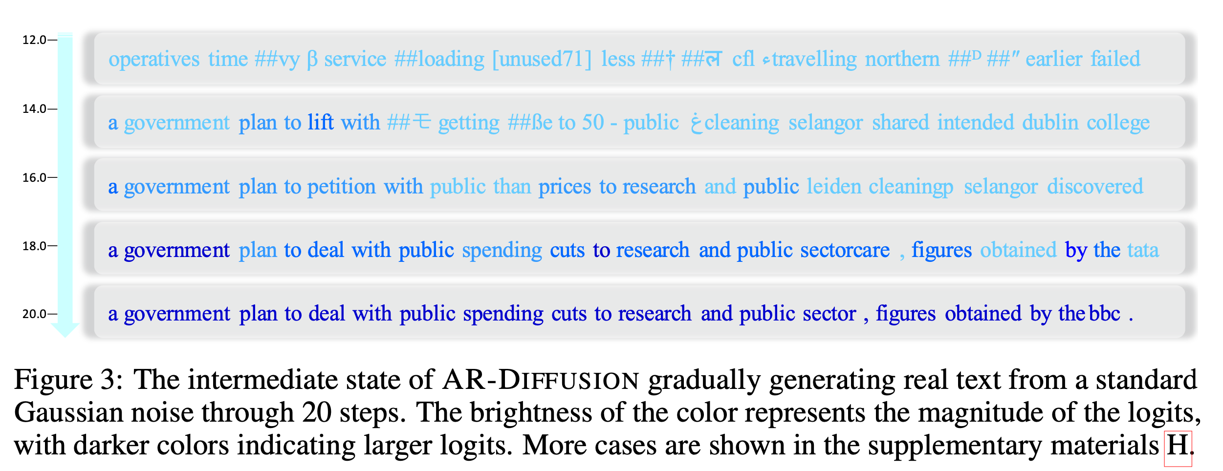
Conclusion
Pure MLE and autoregressive generation are still the way to go for NLG tasks. Some decoding methods, as MCTS guidance or contrastive learning, help to reduce the exposure bias, and are probably the ones giving the best results atow.
Non-autoregressive and gradient-based generation methods usually come with high variance. Many would consider that they comes with too much constraints, and struggle to produce results with both quality and diversity. Diffusion models however benefit from a much better guidance for controllable generation.
This promising area of research might move towards the cooperation between pure MLE models.
References
[1] I. Goodfellow et al., “Generative Adversarial Nets” in Advances in Neural Information Processing Systems, 2014, vol. 27.
[2] A. Holtzman, J. Buys, L. Du, M. Forbes, and Y. Choi, “The Curious Case of Neural Text Degeneration” in ICLR, 2020.
[3] A. Fan, M. Lewis, and Y. Dauphin, “Hierarchical Neural Story Generation” in Proceedings of the 56th Annual Meeting of the Association for Computational Linguistics (Volume 1: Long Papers), Jul. 2018, pp. 889–898. doi: 10.18653/v1/P18-1082.
[4] X. Lu, P. West, R. Zellers, R. Le Bras, C. Bhagavatula, and Y. Choi, “NeuroLogic Decoding: (Un)supervised Neural Text Generation with Predicate Logic Constraints” in Proceedings of the 2021 Conference of the North American Chapter of the Association for Computational Linguistics: Human Language Technologies, Jun. 2021, pp. 4288–4299.
[5] X. Lu et al., “NeuroLogic A*esque Decoding: Constrained Text Generation with Lookahead Heuristics” in Proceedings of the 2022 Conference of the North American Chapter of the Association for Computational Linguistics: Human Language Technologies, Jul. 2022, pp. 780–799.
[6] P. E. Hart, N. J. Nilsson, and B. Raphael, “A Formal Basis for the Heuristic Determination of Minimum Cost Paths” IEEE Transactions on Systems Science and Cybernetics, vol. 4, no. 2, pp. 100–107, 1968.
[7] T. Karras, S. Laine, and T. Aila, “A Style-Based Generator Architecture for Generative Adversarial Networks” in CVPR, Jul. 2019.
[8] J. Engel, K. K. Agrawal, S. Chen, I. Gulrajani, C. Donahue, and A. Roberts, “GANSynth: Adversarial Neural Audio Synthesis” arXiv, 2019.
[9] A. Shoshan, N. Bhonker, I. Kviatkovsky, and G. Medioni, “GAN-Control: Explicitly Controllable GANs” in ICCV, Oct. 2021, pp. 14083–14093.
[10] M. Lee and J. Seok, “Controllable Generative Adversarial Network” IEEE Access, vol. 7, pp. 28158–28169, 2019, doi: 10.1109/ACCESS.2019.2899108.
[11] T. Che et al., “Your GAN is Secretly an Energy-based Model and You Should Use Discriminator Driven Latent Sampling” in Advances in Neural Information Processing Systems, 2020, vol. 33, pp. 12275–12287.
[12] A. F. Ansari, M. L. Ang, and H. Soh, “Refining Deep Generative Models via Discriminator Gradient Flow” in ICLR, 2021.
[13] M. Arjovsky, S. Chintala, and L. Bottou, “Wasserstein GAN” arXiv, 2017.
[14] E. Jang, S. Gu, and B. Poole, “Categorical Reparameterization with Gumbel-Softmax” in ICLR, 2017.
[15] C. J. Maddison, D. Tarlow, and T. Minka, “A* Sampling” in Advances in Neural Information Processing Systems, 2014, vol. 27.
[16] D. P. Kingma, T. Salimans, and M. Welling, “Variational Dropout and the Local Reparameterization Trick” in Advances in Neural Information Processing Systems, 2015, vol. 28.
[17] M. J. Kusner and J. M. Hernández-Lobato, “GANS for Sequences of Discrete Elements with the Gumbel-softmax Distribution” arXiv, 2016.
[18] W. Nie, N. Narodytska, and A. Patel, “RelGAN: Relational Generative Adversarial Networks for Text Generation” in ICLR, 2019.
[19] L. Chen et al., “Adversarial Text Generation via Feature-Mover’s Distance” in Advances in Neural Information Processing Systems, 2018, vol. 31.
[20] L. Yu, W. Zhang, J. Wang, and Y. Yu, “SeqGAN: Sequence Generative Adversarial Nets with Policy Gradient” in Proceedings of the Thirty-First AAAI Conference on Artificial Intelligence, 2017, pp. 2852–2858.
[21] N. De Cao and T. Kipf, “MolGAN: An implicit generative model for small molecular graphs”, arXiv, 2018.
[22] C. de Masson d’Autume, S. Mohamed, M. Rosca, and J. Rae, “Training Language GANs from Scratch” in Advances in Neural Information Processing Systems, 2019, vol. 32.
[23] K. Lin, D. Li, X. He, Z. Zhang, and M. Sun, “Adversarial Ranking for Language Generation” in Advances in Neural Information Processing Systems, 2017, vol. 30.
[24] G. Tucker, A. Mnih, C. J. Maddison, J. Lawson, and J. Sohl-Dickstein, “REBAR: Low-variance, unbiased gradient estimates for discrete latent variable models” in Advances in Neural Information Processing Systems, 2017, vol. 30.
[25] Y. Cong, M. Zhao, K. Bai, and L. Carin, “GO Gradient for Expectation-Based Objectives” in ICLR, 2019.
[26] Y. Cong, M. Zhao, J. Li, J. Chen, and L. Carin, “GO Hessian for Expectation-Based Objectives” Proceedings of the AAAI Conference on Artificial Intelligence, vol. 35, no. 13, pp. 12060–12068, May 2021.
[27] M. Morrison, R. Kumar, K. Kumar, P. Seetharaman, A. Courville, and Y. Bengio, “Chunked Autoregressive GAN for Conditional Waveform Synthesis” in ICLR 2022.
[28] N. Kalchbrenner et al., “Efficient Neural Audio Synthesis” in Proceedings of the 35th International Conference on Machine Learning, Jul. 2018, vol. 80, pp. 2410–2419.
[29]W. Ping, K. Peng, K. Zhao, and Z. Song, “WaveFlow: A Compact Flow-based Model for Raw Audio” in Proceedings of the 37th International Conference on Machine Learning, Jul. 2020, vol. 119, pp. 7706–7716.
[30] M. Caccia, L. Caccia, W. Fedus, H. Larochelle, J. Pineau, and L. Charlin, “Language GANs Falling Short” in ICLR, 2020.
[31] S. Welleck, I. Kulikov, S. Roller, E. Dinan, K. Cho, and J. Weston, “Neural Text Generation With Unlikelihood Training” 2020.
[32] M. Norouzi et al., “Reward Augmented Maximum Likelihood for Neural Structured Prediction,” in Advances in Neural Information Processing Systems, 2016, vol. 29.
[33] J. Su, J. Xu, X. Qiu, and X. Huang, “Incorporating Discriminator in Sentence Generation: a Gibbs Sampling Method,” in AAAI Conference, 2018, doi: 10.1609/aaai.v32i1.11990.
[34] A. Holtzman, J. Buys, M. Forbes, A. Bosselut, D. Golub, and Y. Choi, “Learning to Write with Cooperative Discriminators” in Proceedings of the 56th Annual Meeting of the Association for Computational Linguistics (Volume 1: Long Papers), Jul. 2018, pp. 1638–1649. doi: 10.18653/v1/P18-1152.
[35] T. Scialom, P.-A. Dray, S. Lamprier, B. Piwowarski, and J. Staiano, “Discriminative Adversarial Search for Abstractive Summarization” in Proceedings of the 37th International Conference on Machine Learning, Jul. 2020, vol. 119, pp. 8555–8564.
[36] T. Scialom, P.-A. Dray, J. Staiano, S. Lamprier, and B. Piwowarski, “To Beam Or Not To Beam: That is a Question of Cooperation for Language GANs” in Advances in Neural Information Processing Systems, 2021, vol. 34, pp. 26585–26597.
[37] Lamprier, S., Scialom, T., Chaffin, A., Claveau, V., Kijak, E., Staiano, J., & Piwowarski, B. (2022). “Generative Cooperative Networks for Natural Language Generation” In Proceedings of the 39th International Conference on Machine Learning (Vol. 162, pp. 11891–11905).
[38] A. Chaffin et al., “Which Discriminator for Cooperative Text Generation?” arXiv preprint arXiv:2204.11586, 2022.
[39] P. F. Christiano, J. Leike, T. Brown, M. Martic, S. Legg, and D. Amodei, “Deep Reinforcement Learning from Human Preferences” in Advances in Neural Information Processing Systems, 2017, vol. 30.
[40] L. Ouyang et al., Training language models to follow instructions with human feedback. 2022.
[41] J. W. Rae et al., Scaling Language Models: Methods, Analysis & Insights from Training Gopher. 2022.
[42] E. J. Hu et al., “LoRA: Low-Rank Adaptation of Large Language Models”, ICLR 2022.
[43] A. Glaese et al., Improving alignment of dialogue agents via targeted human judgements, 2022.
[44] Y. Bai et al., Training a Helpful and Harmless Assistant with Reinforcement Learning from Human Feedback 2022.
[45] Rafael Rafailov, undefined., et al, Direct Preference Optimization: Your Language Model is Secretly a Reward Model in ICML 2023 Workshop The Many Facets of Preference-Based Learning, 2023.
[46] Lewis, P., et al, Retrieval-Augmented Generation for Knowledge-Intensive NLP Tasks in Advances in Neural Information Processing Systems, 2020, pp. 9459–9474.
[47] Y. Su, T. Lan, Y. Wang, D. Yogatama, L. Kong, and N. Collier, “CoNT: Contrastive Neural Text Generation” in Advances in Neural Information Processing Systems, 2022, vol. 35.
[48] Y. Su, T. Lan, Y. Wang, D. Yogatama, L. Kong, and N. Collier, “A Contrastive Framework for Neural Text Generation” in Advances in Neural Information Processing Systems, 2022.
[49] Kawin Ethayarajh, How Contextual are Contextualized Word Representations? Comparing the Geometry of BERT, ELMo, and GPT-2 Embeddings, in EMNLP 2019.
[50] Xingyu Cai, Jiaji Huang, Yuchen Bian, and Kenneth Church. 2021. Isotropy in the Contextual Embedding Space: Clusters and Manifolds in ICLR 2022.
[51] X. L. Li et al., Contrastive Decoding: Open-ended Text Generation as Optimization. arXiv, 2022. doi: 10.48550/ARXIV.2210.15097.
[52] Xu, N., et al, Look-back Decoding for Open-Ended Text Generation in Proceedings of the 2023 Conference on Empirical Methods in Natural Language Processing, 2023, pp. 1039–1050.
[53] Min, S., et al, Nonparametric Masked Language Modeling in Findings of the Association for Computational Linguistics: ACL 2023, 2023, pp. 2097–2118.
[54] J. Ho, A. Jain, and P. Abbeel, “Denoising Diffusion Probabilistic Models” in Advances in Neural Information Processing Systems, 2020, vol. 33, pp. 6840–6851.
[55] Y. Song and S. Ermon, “Generative Modeling by Estimating Gradients of the Data Distribution” in Advances in Neural Information Processing Systems, 2019, vol. 32.
[56] J. Sohl-Dickstein, E. Weiss, N. Maheswaranathan, and S. Ganguli, “Deep Unsupervised Learning using Nonequilibrium Thermodynamics” in Proceedings of the 32nd International Conference on Machine Learning, Jul. 2015, vol. 37, pp. 2256–2265.
[57] L. Qin, S. Welleck, D. Khashabi, and Y. Choi, “COLD decoding: Energy-based constrained text generation with langevin dynamics” arXiv preprint arXiv:2202.11705, 2022.
[58] E. Hoogeboom, D. Nielsen, P. Jaini, P. Forré, and M. Welling, “Argmax Flows and Multinomial Diffusion: Learning Categorical Distributions” in Advances in Neural Information Processing Systems, 2021, vol. 34, pp. 12454–12465.
[59] J. Austin, D. D. Johnson, J. Ho, D. Tarlow, and R. van den Berg, “Structured Denoising Diffusion Models in Discrete State-Spaces” in Advances in Neural Information Processing Systems, 2021, vol. 34, pp. 17981–17993.
[60] X. Li, J. Thickstun, I. Gulrajani, P. S. Liang, and T. B. Hashimoto, “Diffusion-LM Improves Controllable Text Generation” in Advances in Neural Information Processing Systems, 2022, vol. 35, pp. 4328–4343.
[61] J. Chen, A. Zhang, M. Li, A. Smola, and D. Yang, “A Cheaper and Better Diffusion Language Model with Soft-Masked Noise”, EMNLP 2023.
[62] S. Gong, M. Li, J. Feng, Z. Wu, and L. Kong, “DiffuSeq: Sequence to Sequence Text Generation with Diffusion Models” ICLR 2023.
[63] Lin, Z., et al, “Text Generation with Diffusion Language Models: A Pre-training Approach with Continuous Paragraph Denoise” in Proceedings of the 40th International Conference on Machine Learning, 2023, pp. 21051–21064.
[64] Singh, M., et al, CodeFusion: A Pre-trained Diffusion Model for Code Generation in Proceedings of the 2023 Conference on Empirical Methods in Natural Language Processing, 2023, pp. 11697–11708.
[65] Emiel Hoogeboom, undefined., et al, “Autoregressive Diffusion Models” in International Conference on Learning Representations, 2022.
[66] X. Han, S. Kumar, Y. Tsvetkov, “SSD-LM: Semi-autoregressive Simplex-based Diffusion Language Model for Text Generation and Modular Control” in Proceedings of the 61st Annual Meeting of the Association for Computational Linguistics (Volume 1: Long Papers), 2023, pp. 11575–11596.
[67] Rabeeh Karimi Mahabadi, undefined., et al, “TESS: Text-to-Text Self-Conditioned Simplex Diffusion” 2023.
[68] Tong Wu, undefined., et al, “AR-Diffusion: Auto-Regressive Diffusion Model for Text Generation” in Thirty-seventh Conference on Neural Information Processing Systems, 2023.